


The experimental framework outlines a comprehensive approach for privacy-preserving medical image classification using federated learning. This framework integrates advanced deep learning models, efficient data preprocessing techniques, and adaptive aggregation methodologies to address the challenges posed by heterogeneous and non-IID medical data distributions across multiple clients. The framework is designed to leverage the strengths of transfer learning architectures while ensuring data privacy and scalability.

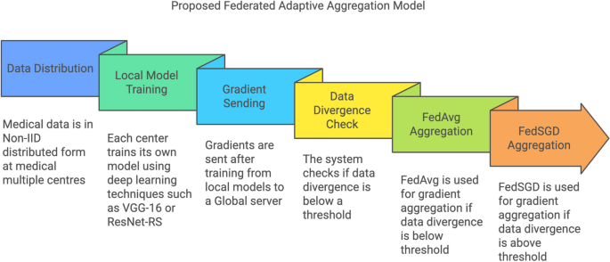
Flowchart depicting the workflow of the proposed federated adaptive aggregation model.
The flowchart in Fig. 3 illustrates the workflow of the proposed federated adaptive aggregation model for privacy-preserving medical image classification. The process begins with the non-IID distribution of medical data across multiple clients, simulating real-world scenarios where data is inherently heterogeneous. Each client trains a local model using deep learning techniques such as VGG-16 or ResNet-RS, tailored to the assigned subset of the dataset.
Once the local training is complete, gradients are transmitted to the central server, initiating the global aggregation process. A divergence check is performed to evaluate the variability in data distributions across clients. Based on the divergence threshold the system dynamically selects the appropriate aggregation method. If the divergence is below the threshold, FedAvg is employed for computationally efficient aggregation. Conversely, if the divergence exceeds the threshold, FedSGD is utilized to preserve performance by incorporating finer gradient updates.
This adaptive framework ensures scalability, robustness, and efficient utilization of resources, addressing the challenges posed by non-IID data distributions in federated learning environments.
The subsequent subsections detail the key components of the framework, starting with data distribution and preprocessing, followed by the customization of transfer learning models, the implementation of federated learning techniques, and the evaluation metrics used to assess model performance. Each component plays a vital role in building a robust and efficient system for decentralized medical image classification.
Data and preprocessing
The datasets included in this study were obtained from publically accessible platforms like Kaggle, offering a varied collection of medical images crucial for assessing the efficacy of the chosen models. Table 2 shows the details of all the three datasets used for this research. The TB chest X-ray dataset comprises 7000 pictures and 2 classes, evenly divided between 3500 normal chest X-rays and 3500 X-rays suggestive of tuberculosis. This dataset facilitates the models’ ability to differentiate between healthy and tuberculosis-affected cases, an essential function in tuberculosis detection. The sample images from the dataset can be seen in the Fig. 4

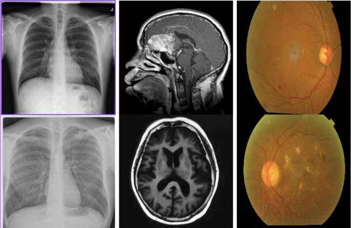
Sample images of all the datasets utilized in this study.
The diabetic retinopathy dataset comprises 3662 JPEG photos, classified into five classes as No DR, Mild, Moderate, Severe, and ProliferateDR, which denote different stages of diabetic retinopathy. This dataset facilitates the classification of various disease phases, enhancing early diagnosis and intervention options in diabetes patients.
The brain tumour dataset comprises 3624 JPEG photos categorised into four classes as no tumour, meningioma, glioma, and pituitary tumour. This dataset offers a variety of brain MRI images essential for tumour type classification, crucial for treatment planning and clinical decision-making.
Each dataset is randomly distributed across 10 clients in a non-IID manner, simulating real-world scenarios where different medical institutions have localized and diverse data. This distribution strategy ensures that clients receive subsets of the data with inherent variability, such as specific classes or regional differences. For example, one client might predominantly have “Normal” TB X-rays, while another might have a higher proportion of “TB” cases, reflecting realistic heterogeneity in data availability. Federated learning in real-world applications often suffers from performance degradation due to Non-IID data distribution across clients. Recent work, such as FedPIA27, has proposed optimization strategies leveraging parameter importance to mitigate local-global divergence, highlighting the need for adaptive aggregation approaches in federated setups.
The datasets are divided into training, validation, and testing subsets with proportions of 70%, 15%, and 15%, respectively. This partitioning ensures that sufficient data is available for model training, hyperparameter tuning, and final performance evaluation. Each image is resized to \(224 \times 224\) pixels and normalized to the range [0, 1], providing a standardized input format for transfer learning models. These preprocessing steps ensure compatibility across all datasets and maintain consistency in model input.
To ensure clarity and consistency throughout the manuscript, the parameters and notations used in the proposed framework are summarized in Table 3. These parameters are integral to describing the federated learning methodology and its components, including local and global model updates, divergence measurements, and aggregation processes.
Stratified non-IID data distribution and preprocessing
Initially, datasets were randomly distributed across multiple clients to simulate decentralized medical environments. However, such an allocation may not adequately represent real-world scenarios where data across institutions is inherently heterogeneous in terms of disease prevalence, data volume, and imaging quality. Therefore, a refined stratified non-IID data allocation method was employed to closely mirror practical multi-institutional settings.
Specifically, the revised data allocation strategy explicitly accounts for realistic variability encountered in medical institutions by considering three key aspects:
-
Disease prevalence: Each client received datasets with varying prevalence rates of diseases, reflecting actual differences among medical institutions.
-
Data volume: The number of images allocated to each client varied, mimicking differences in institutional resources and patient intake.
-
Image quality: To simulate realistic discrepancies in imaging capabilities and diagnostic quality, datasets varied slightly in image resolution and incorporated controlled noise where appropriate.
Table 4 summarizes the refined dataset distribution among the 10 clients.
All images were resized to a standard dimension of 224 \(\times\) 224 pixels and normalized to a range of [0, 1] to maintain consistency in model inputs despite variability in data quality. This refined strategy ensures a realistic evaluation scenario, effectively testing the robustness and adaptability of the federated learning framework.
Benchmarking the proposed framework with baseline models
To evaluate the efficacy of the proposed adaptive aggregation methodology, comprehensive benchmarking was conducted using baseline models and modern architectures. This section presents a detailed analysis of the models’ performance across multiple datasets and aggregation methods, highlighting the strengths and weaknesses of each approach. The results are analyzed to assess the impact of adaptive aggregation on accuracy, efficiency, and resource utilization.
The fine-tuning and validation of the pre-trained models GoogLeNet and VGG16 were essential elements of the transfer learning methodology employed for medical picture categorisation. The datasets utilised were partitioned into training, validation, and testing sets, with 70% designated for training, 15% for validation, and the remaining 15% for testing. The equitable distribution was crucial to guarantee that the models were sufficiently trained while upholding a just assessment during the validation and testing stages.
Fine-tuning entailed modifying the weights of the pre-trained models, which were initially trained on ImageNet, to accommodate the specific medical picture datasets utilised. The foundational layers of the models, which encapsulate fundamental features like edges and textures, were predominantly preserved, whereas the superior layers were refined to identify domain-specific characteristics pertinent to medical imaging, including anomaly detection in TB chest X-rays, brain tumour segmentation, and classification of diabetic retinopathy stages. This technique facilitated the fast acquisition of medical-specific patterns without necessitating the training of models from the ground up, thus minimising computational time and resource requirements.
During training, the models were iteratively updated using backpropagation and gradient descent. The model parameters \(\textbfD_k\) were optimized by minimizing the categorical cross-entropy loss \(\mathscr \), which is defined for multi-class classification as:
$$\begin \mathscr (\textbf) = – \sum _^D_k \sum _^{C} y_{i,c} \log (\hat{y}_{i,c}) \end{aligned}$$
(1)
where \(N\) is the number of training samples, \(C\) is the number of classes, \(y_{i,c}\) is the true label of class \(c\) for sample \(i\), and \(\hat{y}_{i,c}\) is the predicted probability for class \(c\).
It computes the categorical cross-entropy loss \(\mathscr {L}(\textbf{w})\), which measures the difference between the predicted probability distribution (\(\hat{y}\)) and the true labels (\(y\)) for all training samples. The output represents the overall error in the model’s predictions, serving as a scalar value that the training process aims to minimize.
The gradients of the loss function with respect to the parameters were computed, and the model was updated using gradient descent:
$$\begin{aligned} \textbf{w}^{(t+1)} = \textbf{w}^{(t)} – \eta \nabla \mathscr {L}(\textbf{w}^{(t)}) \end{aligned}$$
(2)
where \(\eta\) is the learning rate, and \(\nabla \mathscr {L}(\textbf{w}^{(t)})\) represents the gradient of the loss function at iteration \(t\).
It computes the updated model parameters \(\textbf{w}^{(t+1)}\) by adjusting the previous parameters \(\textbf{w}^{(t)}\) in the direction of the negative gradient. The output represents the refined model parameters after one iteration of training, moving the model closer to minimizing the loss.
To prevent overfitting, regularization techniques such as dropout were applied during training. In dropout, a fraction \(p\) of the neurons in each layer were randomly set to zero during each iteration, effectively reducing the complexity of the model. Additionally, early stopping was employed to halt training when the validation loss did not improve after a set number of epochs, thus preventing overfitting.
The validation set was used to monitor the performance of the models during training, ensuring that the fine-tuning process did not lead to overfitting or underfitting.
VGG 16 model

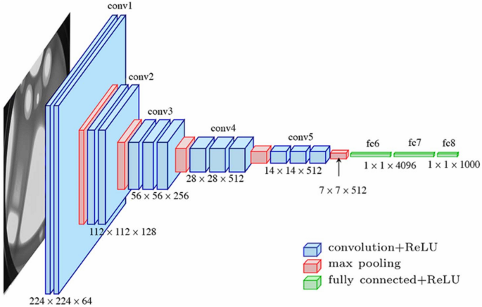
VGG-16 architecture as introduced in28.
The VGG16 model was utilized for medical image classification due to its depth and robust feature extraction capabilities29. VGG16, with its 16 layers as shown in Fig. 5, is well-suited for learning detailed hierarchical features in medical images such as TB chest X-rays, brain tumor MRIs, and diabetic retinopathy images30. The convolutional layers in VGG16 use fixed-sized filters (3 \(\times\) 3) to extract features from input images, which can be represented as:
$$\begin{aligned} \textbf{y}_{i,j} = \sum _{m=1}^{M} \sum _{n=1}^{N} \textbf{w}_{m,n} \textbf{x}_{i+m, j+n} + b, \quad \textbf{x} \in \{D_k^{\text {TB}}, D_k^{\text {MRI}}, D_k^{\text {DR}}\} \end{aligned}$$
(3)
where \(\textbf{x}\) represents the input image from one of the medical datasets TB chest X-rays, brain tumor MRIs, or diabetic retinopathy images, \(\textbf{w}\) is the convolutional filter, \(b\) is the bias, and \(\textbf{y}\) is the output feature map. This equation computes the feature map \(\textbf{y}\) by applying the convolutional filter \(\textbf{w}\) over the input image \(\textbf{x}\), extracting spatial features such as edges and textures essential for subsequent layers.
This systematic convolution over medical images allows VGG16 to capture both low-level and high-level features critical for medical diagnosis.
The suitability of VGG16 for this study lies in its ability to capture fine-grained details necessary for the accurate classification of medical conditions. The network’s depth provides the advantage of learning complex patterns from medical images such as small lesions in diabetic retinopathy or subtle tumor regions in brain MRIs. Additionally, VGG16’s architecture, when fine-tuned through transfer learning, was able to generalize well on the medical datasets after being trained on a large dataset like ImageNet, thus reducing the computational cost and training time.
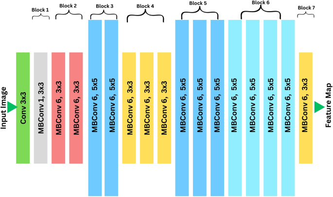
GoogLeNet model

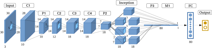
GoogLenet architecture as introduced in31.
The VGG16 model was utilized for medical image classification due to its depth and robust feature extraction capabilities29. VGG16, with its 16 layers as shown in Fig. 5, is well-suited for learning detailed hierarchical features in medical images such as TB chest X-rays, brain tumor MRIs, and diabetic retinopathy images30. The convolutional layers in VGG16 use fixed-sized filters (3 \(\times\) 3) to extract features from input images, which can be represented as:
$$\begin{aligned} \textbf{y}_{i,j} = \sum _{m=1}^{M} \sum _{n=1}^{N} \textbf{w}_{m,n} \textbf{x}_{i+m, j+n} + b, \quad \textbf{x} \in \{D_k^{\text {TB}}, D_k^{\text {MRI}}, D_k^{\text {DR}}\} \end{aligned}$$
(4)
where \(\textbf{x}\) represents the input image from one of the medical datasets (TB chest X-rays, brain tumor MRIs, or diabetic retinopathy images), \(\textbf{w}\) is the convolutional filter, \(b\) is the bias, and \(\textbf{y}\) is the output feature map. This equation computes the feature map \(\textbf{y}\) by applying the convolutional filter \(\textbf{w}\) over the input image \(\textbf{x}\), extracting spatial features such as edges and textures essential for subsequent layers.
This systematic convolution over medical images allows VGG16 to capture both low-level and high-level features critical for medical diagnosis.
The suitability of VGG16 for this study lies in its ability to capture fine-grained details necessary for the accurate classification of medical conditions. The network’s depth provides the advantage of learning complex patterns from medical images such as small lesions in diabetic retinopathy or subtle tumor regions in brain MRIs. Additionally, VGG16’s architecture, when fine-tuned through transfer learning, was able to generalize well on the medical datasets after being trained on a large dataset like ImageNet, thus reducing the computational cost and training time.
GoogLeNet was selected for medical image classification due to its unique architecture as shown in Fig. 6, which efficiently captures multi-scale features through the use of inception modules32. Each inception module processes the input data with multiple filters of different sizes such as 1 \(\times\) 1, 3 \(\times\) 3, 5 \(\times\) 5 convolutions in parallel, allowing GoogLeNet to extract features at various scales simultaneously33. The output of an inception module can be mathematically described as:
$$\begin{aligned} \textbf{y}_{i,j}^{(k)} = \sum _{m=1}^{M_k} \sum _{n=1}^{N_k} \textbf{w}_{m,n}^{(k)} \textbf{x}_{i+m, j+n} + b^{(k)}, \quad \textbf{x} \in \{D_k^{\text {TB}}, D_k^{\text {MRI}}, D_k^{\text {DR}}\} \end{aligned}$$
(5)
where \(k\) denotes the different filter sizes used within the inception module, \(\textbf{x}\) represents the input image from one of the medical datasets (TB chest X-rays, brain tumor MRIs, or diabetic retinopathy images), \(\textbf{w}^{(k)}\) is the filter for each size, and \(\textbf{y}^{(k)}\) is the feature map output for that specific filter. This equation shows how the inception module combines outputs from filters of varying sizes to generate multi-scale feature maps, enabling the model to detect both fine-grained details and large-scale patterns in medical images.
This architecture is particularly suitable for the heterogeneous nature of medical images, such as TB chest X-rays and brain MRIs, which contain both large-scale and fine-grained features.
GoogLeNet’s suitability lies in its ability to simultaneously process multiple feature scales, which is crucial for accurately detecting anomalies like small lesions in diabetic retinopathy or subtle changes in brain MRIs. By leveraging transfer learning, the model was fine-tuned to adapt to medical datasets, ensuring efficient training and robust performance.
GoogLeNet’s ability to process features at different scales made it highly effective in identifying complex patterns, such as small microaneurysms in diabetic retinopathy images or distinct tumor boundaries in brain MRIs. The inception architecture allowed GoogLeNet to reduce the number of parameters compared to deeper models like VGG16, improving computational efficiency without sacrificing accuracy. The suitability of GoogLeNet for this research was further enhanced by its use of global average pooling layers, which replaced the fully connected layers, thus reducing overfitting on the relatively small medical datasets.
While the baseline models VGG16 and GoogLeNet demonstrate robust feature extraction and classification capabilities in centralized environments, the sensitivity of medical image data necessitates additional privacy-preserving measures. To address these concerns, differential privacy is introduced as an integral component of the experimental framework, ensuring that the models can be trained in a secure centralized environment without compromising the confidentiality of individual data points.
Differential privacy
Differential privacy34 was employed in the centralized environment to protect sensitive medical data during the training of the models35,36. Differential privacy provides a mathematical guarantee that the inclusion or exclusion of any single data point will not significantly affect the outcome of the model37, thereby ensuring that individual data points remain private. This was achieved by introducing noise into the gradients during backpropagation, which prevents the model from memorizing specific details about the training data38. The differentially private gradient update can be mathematically expressed as:
$$\begin{aligned} \nabla \mathscr {L}(\textbf{w}) \leftarrow \nabla \mathscr {L}(\textbf{w}; D_k^{\text {TB}}, D_k^{\text {MRI}}, D_k^{\text {DR}}) + \mathscr {N}(0, \sigma ^2) \end{aligned}$$
(6)
where \(\nabla \mathscr {L}(\textbf{w})\) represents the gradient of the loss function \(\mathscr {L}(\textbf{w})\) computed over the medical datasets (TB chest X-rays, brain tumor MRIs, and diabetic retinopathy images), and \(\mathscr {N}(0, \sigma ^2)\) is Gaussian noise with a mean of 0 and variance \(\sigma ^2\), introduced to preserve privacy. The parameter \(\sigma ^2\) controls the scale of the noise, with larger values offering stronger privacy guarantees but potentially impacting the model’s accuracy. The privacy budget \(\epsilon\) governs the level of privacy and defines the trade-off between privacy and model utility. A smaller \(\epsilon\) provides stronger privacy but can reduce the accuracy of the model.
The differentially private model update at each step is given by:
$$\begin{aligned} \textbf{w}_{t+1} = \textbf{w}_t – \eta \left( \nabla \mathscr {L}(\textbf{w}_t; D_k^{\text {TB}}, D_k^{\text {MRI}}, D_k^{\text {DR}}) + \mathscr {N}(0, \sigma ^2) \right) \end{aligned}$$
(7)
where \(\textbf{w}_{t+1}\) is the updated model parameter, \(\textbf{w}_t\) is the previous parameter, and \(\eta\) is the learning rate. By adding controlled noise to the gradient during each update, the model ensures that even if a malicious actor gains access to the model’s parameters, they cannot infer details about any individual data point. This method was particularly important for ensuring privacy in the centralized training of medical images, where the sensitivity of personal health information requires strong protection mechanisms.
Differential privacy was used to balance the trade-off between accuracy and privacy in the centralized environment. While the noise addition may introduce some loss in accuracy, it ensures that the trained model maintains privacy guarantees that are critical when dealing with sensitive medical datasets like TB chest X-rays, brain tumor MRI scans, and diabetic retinopathy images.
Although differential privacy provides a robust mechanism for protecting data in centralized environments, the limitations of centralization in multi-institutional settings necessitate a federated approach. The federated learning setup leverages decentralized data stored across multiple medical centers, ensuring privacy preservation by eliminating the need to share raw data. This section outlines the structure of the federated learning environment, detailing the adaptive aggregation techniques employed to address challenges arising from non-IID data distributions.
Federated learning setup
A federated learning setup is employed to ensure privacy-preserving medical image classification, wherein the local data from different clients is trained without sharing the raw data with the central server. To improve the efficiency and accuracy of the global model, an adaptive aggregation methodology is introduced, which dynamically selects between FedAvg39,40 and FedSGD41,42 based on the divergence of data across clients.
The medical image data is distributed across 10 clients in a non-IID manner, ensuring that each client has access to a random subset of the dataset. This non-IID43,44 setup reflects real-world conditions where different medical institutions or devices may have data with varying distributions. The local model on each client k, denoted as \(w_k^t\), is updated by performing local training using SGD, where the model parameters are updated as follows:
$$\begin{aligned} w_k^{t} = w_k^{t-1} – \eta \nabla L_k(w_k^{t-1}; D_k^{\text {TB}}, D_k^{\text {MRI}}, D_k^{\text {DR}}) \end{aligned}$$
(8)
Here, \(w_k^{t}\) represents the local model parameters of client k at iteration t, and \(D_k^{\text {TB}}, D_k^{\text {MRI}}, D_k^{\text {DR}}\) are the subsets of the TB chest X-ray, brain tumor MRI, and diabetic retinopathy datasets, respectively. This equation computes the updated local model parameters after each iteration of training on client k, reflecting the gradients computed on the client’s local data.
Once the local models have been trained on their respective datasets, the global model needs to be updated. The adaptive aggregation methodology is employed at this stage to optimize the communication and model update process. If the divergence across clients’ model updates is high, indicating substantial variation in local data distributions, Federated SGD is utilized for aggregation. This is mathematically expressed as:
$$\begin{aligned} w_t = w_{t-1} – \eta \sum _{k=1}^{K} \frac{|D_k|}{N} \nabla L_k(w_{t-1}) \end{aligned}$$
(9)
where \(w_t\) is the global model at round t, K is the number of clients, \(|D_k|\) is the number of data points in client k’s local dataset, and \(N = \sum _{k=1}^{K} |D_k|\) is the total number of data points across all clients. This equation computes the updated global model parameters by aggregating gradients from all clients, ensuring the model reflects the diverse data distributions more accurately in cases of high divergence.
However, when the divergence between the client models is low or moderate, FedAvg is used as a more efficient method for aggregation. FedAvg averages the locally updated models and combines them into the global model, which can be expressed as:
$$\begin{aligned} w_t = \sum _{k=1}^{K} \frac{|D_k|}{N} w_k^{t} \end{aligned}$$
(10)
Here, each client’s contribution to the global model is weighted by the size of their local dataset. This equation shows how the global model is updated by averaging the local models, making FedAvg computationally less demanding compared to FedSGD and suitable for rounds with lower divergence.
The decision between FedSGD and FedAvg is made by dynamically evaluating the divergence \(\delta _t\) across client models. The divergence is measured as the average distance between the local models and the global model, defined as:
$$\begin{aligned} \delta _t = \frac{1}{K} \sum _{k=1}^{K} \left\| w_k^{t} – w_t \right\| _2, \quad D_k \in \{\text {TB, MRI, DR}\} \end{aligned}$$
(11)
If \(\delta _t\) exceeds a predefined threshold \(\tau\), indicating high divergence, FedSGD is used for aggregation to allow for finer updates based on gradients. Conversely, if \(\delta _t \le \tau\), FedAvg is used to aggregate the models more efficiently. This equation computes the divergence between client models and the global model, which is then used to decide the aggregation strategy, optimizing the communication process and ensuring the most appropriate method is employed for the current state of divergence across clients.
By dynamically switching between FedAvg and FedSGD, this methodology ensures that the global model is updated efficiently while accounting for the varying levels of divergence in the data across clients. This approach improves both the computational efficiency and the accuracy of the global model, especially in a non-IID data distribution setup, where divergence can significantly affect model convergence and performance. The algorithm for the proposed FL framework for medical multi-center image classification and secure data analysis can be given as:

Federated learning with adaptive aggregation in non-IID multiple medical centers setup.
Incorporating modern architectures into the proposed framework
To further enhance the performance and scalability of the proposed federated learning framework, modern deep learning architectures such as EfficientNetV2 and ResNet-RS are evaluated alongside the baseline models. These architectures are specifically designed to optimize resource utilization and handle complex datasets, making them well-suited for privacy-preserving medical image classification in federated environments. The following subsection presents the evaluation of these modern architectures, highlighting their contributions to the overall framework.
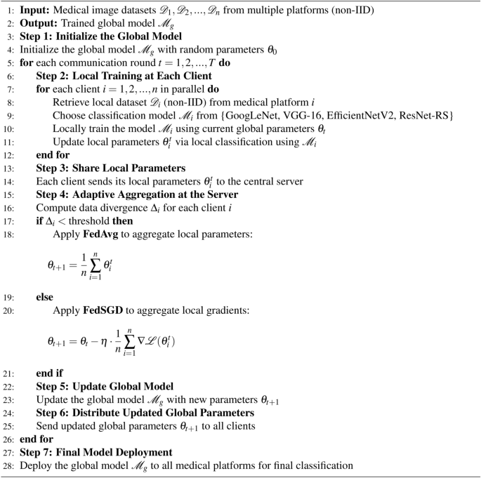
EfficientNetV2

EfficientNetV2 architecture.
EfficientNetV2 is a state-of-the-art convolutional neural network architecture designed for efficient scaling and optimal performance in image classification tasks45. It employs a compound scaling method to balance the depth (d), width (w), and resolution (r) of the network, ensuring a trade-off between accuracy and computational cost46. The detailed architecture of EfficientNetV2 is shown in Fig. 7. The scaling is mathematically defined as:
$$\begin{aligned} r = \alpha ^k, \quad w = \beta ^k, \quad d = \gamma ^k, \quad \text {subject to } \alpha \cdot \beta ^2 \cdot \gamma ^2 \approx 2, \end{aligned}$$
(12)
where \(\alpha\), \(\beta\), and \(\gamma\) are scaling coefficients, and k is the scaling factor. This equation computes the scaling factors for resolution (r), width (w), and depth (d) of the network, ensuring uniform scaling across dimensions to effectively handle high-resolution medical images without excessive computational overhead47.
EfficientNetV2 utilizes inverted residual blocks, which are mathematically represented as:
$$\begin{aligned} y = \sigma (BN(W \cdot x)), \quad x \in \{D_k^{\text {TB}}, D_k^{\text {DR}}\} \end{aligned}$$
(13)
where x is the input tensor from datasets such as TB chest X-rays or diabetic retinopathy images, W represents the convolutional weights, BN denotes batch normalization, and \(\sigma\) is the activation function. This equation computes the output tensor y by applying convolutional operations followed by batch normalization and activation, enabling the network to extract hierarchical features critical for medical image classification.
These architectural improvements make EfficientNetV2 particularly suitable for federated learning environments, where communication efficiency and scalability are crucial. In this experiment, EfficientNetV2 was employed to handle datasets such as TB chest X-rays and diabetic retinopathy images due to its ability to extract fine-grained features, adapt to non-IID data distributions, and converge faster in decentralized setups. These characteristics align with the need to minimize communication costs while achieving high classification accuracy across multiple clients.
ResNet-RS

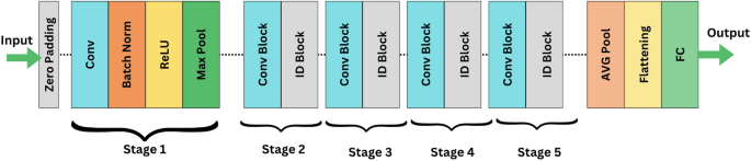
ResNet-RS, an advanced adaptation of the ResNet architecture, was also utilized for medical image classification. This model introduces improved scaling strategies and training optimizations, making it highly efficient for handling complex datasets in contemporary hardware environments48. The detailed architecture of ResNet-RS is shown in Fig. 8. ResNet-RS retains the use of residual blocks to mitigate vanishing gradient issues, represented as:
$$\begin{aligned} y = \sigma (F(x, \{W_i\}) + x), \quad x \in \{D_k^{\text {MRI}}, D_k^{\text {DR}}\} \end{aligned}$$
(14)
where \(F(x, \{W_i\})\) is the residual mapping, x represents the input from datasets such as brain tumor MRI and diabetic retinopathy images, \(W_i\) are the convolutional weights, and \(\sigma\) is the activation function. This equation computes the output tensor y by adding the residual mapping \(F(x, \{W_i\})\) to the input tensor x, enabling the network to retain previously learned features while learning new hierarchical features crucial for accurate classification.
These skip connections enable deeper networks to converge more effectively, making ResNet-RS particularly robust in extracting hierarchical features from multi-class datasets49. In this study, ResNet-RS was applied to datasets such as brain tumor MRI and diabetic retinopathy images, where its robustness in distinguishing overlapping features and rare classes significantly improved classification performance50.
Both EfficientNetV2 and ResNet-RS were integrated into the federated learning framework to leverage their complementary strengths. In this setup, models were trained locally on client devices, with global aggregation performed using adaptive methods such as FedAvg and FedSGD. The global model weights \(\theta _G\) were updated iteratively using the equation:
$$\begin{aligned} \theta _G^{(t+1)} = \sum _{i=1}^N \frac{n_i}{n} \cdot \theta _i^{(t)}, \quad n = \sum _{i=1}^N n_i \end{aligned}$$
(15)
where N represents the total number of clients, \(n_i\) is the number of samples on the i-th client, and \(\theta _i^{(t)}\) denotes the local model weights after t iterations. This equation computes the updated global model weights \(\theta _G^{(t+1)}\) by aggregating the weighted contributions of local model parameters from all clients, ensuring that the global model reflects the diversity of client data.
EfficientNetV2’s ability to efficiently process high-resolution images and ResNet-RS’s capacity to extract complex features ensured that the federated framework performed robustly across diverse datasets while preserving data privacy. These models not only have the ability to reduce local training errors but also improve the overall convergence rate, highlighting their suitability for privacy-preserving collaborative learning in multi-institutional settings.
link