
Anomaly-based threat detection in smart health using machine learning | BMC Medical Informatics and Decision Making

This study examines the challenges in safeguarding sensitive EHR. Rapid technology integration necessitates fortifying EHRs against insider threats to ensure patient privacy and data integrity. In this research we have utilized a dataset from a hospital in North England. The data contains information related to patients under treatment in the hospital.
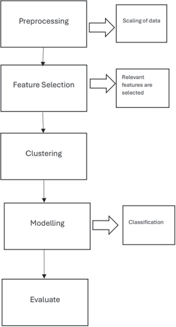
Flow diagram of proposed methodology
The Fig. 3 depicts various steps of the flow diagram and the Fig. 4 shows details of different phases of the methodology adopted. Firstly in the pre processing phase, data is cleaned and prepared for the analysis. Afterwards feature selection techniques including correlation analysis is carried out to include only the related features . As the data is unlabelled , we utilized two popular algorithms including the isolation forest and local outlier factor. The data is labelled and is validated by utilization of the anomaly scores and other metrics. Finally the model is trained utilizing the supervised algorithms. Thus the methodology is able to predict any unknown instance as anomalous or vice versa.

Dataset
This study has utilized a dataset of electronic health records (EHRs) [51]. The dataset consists of 1,007,727 entries from the audit logs. The dataset contains EHR of patient data, medical histories and other information as given in the Table 1. The data belongs to a hospital in North England.
Preprocessing phase
This phase consists of three main stages including data cleaning, missing values management and normalization. Numeric missing values are replaced with the mean value, while the nominal missing values are replaced with the mode. Categorical data is converted into numerical representation through One-hot encoding. Normalization is done using the min-max algorithm, adjusting numeric values to a range between 0 and 1 [52].
To ensure the data is suitably prepared for further analysis and modeling, these meticulous steps are implemented, resulting in outcomes that are more accurate and reliable.
$$\beginN_k(p) \text N_k(p)norm = \frac{lrd_k(p) \cdot }{{\text {max}(x) – \text {min}(x)}} \end{aligned}$$
(1)
The min-max algorithm, outlined in Eq. 1 in [53], is applied to numeric values to standardize them within the range of 0 to 1, facilitating easier comparison between different variables.
Labeling phase
Post-data refinement, a total of 90,385 distinct identifiers were discerned. Employing a cross-correlation examination, we performed feature selection. Subsequently, we partitioned the dataset into training and evaluation subsets, deploying assorted clustering methodologies. A comparative analysis of clustering efficacy between Isolation Forest and Local Outlier Factor (LOF) was conducted. Ultimately, the validity of outlier ratings derived from the clustering procedure was verified.
Cross correlation
Cross-correlation proves advantageous in scenarios where interrelations exist among dataset features, allowing exploitation of these associations. Consequently, a segment of the data remains untapped, resulting in reduced data volume and computational intricacy. The formula employed to ascertain the cross-correlation between two sequences, u(n) and h(n), is delineated as follows:
$$\begin{aligned} \text {Cross-correlation} = \sum \limits _{n} u(n) \cdot h(n – k) \end{aligned}$$
(2)
where: \(u(n)\) represents the values of the first sequence at time \(n\),
\(h(n – k)\) represents the values of the second sequence shifted by \(k\) time units.
According to Eq. 2 cited in [54], the peak cross-correlation occurs when two sequences, represented as \(u(n)\) and \(h(n)\), are identical. This cross-correlation concept is widely applied across various domains, notably in network intrusion detection. Presented here is an overview of several methodologies leveraging cross-correlation for the identification of network intrusions. Researchers [55, 56] have utilized cross correlation as a feature selection technique for intrusion detection.
In another study [57], utilization of cross correlation demonstrated improvement in the detection accuracy of intrusion attacks in network traffic.
In the domain of classification and intrusion detection, false correlations among features can arise, posing challenges for intrusion detection systems (IDS). Additionally, redundant information across features may complicate the detection process. The inclusion of unnecessary features can prolong computation time and impact IDS accuracy. Achieving optimal classification accuracy hinges on selecting the most relevant subset of features that accurately classify training data. Cross Correlation aids by identifying redundant features and establishes features that can increase the performance of machine learning models.The cross correlation algorithm works according to the following steps.
1. Firstly an initial set of all features is established.
2. The correlation of feature to feature is calculated according to the Eq. 2.
3. The feature that produces maximum correlation is identified.
4. Iterate through step 2 and 3 until desired features are selected.
Features that have high value of correlation show they are similar, and carry similar information. Thus one of them can be selected. Low value indicates the features are unrelated and they carry different information. In the dataset in this study cross correlation revealed that an important feature of Discharge Date was not taken into account in the baseline approach thus loosing some valuable information.
Clustering-Isolation Forest (IForest)
The isolation forest constructs decision trees to isolate anomalies from normal instances, identifying anomalies as points requiring fewer splits across trees. According to standard 70% of the dataset was used for training purposes and the remaining 30% for testing the models.The clustering algorithm assigns labels to the dataset as anomaly or normal instances.
In summary, the training and testing process with the isolation forest offers a means to detect anomalies in datasets, contributing to the anomaly detection field in machine learning.
Training step
This is the stage where the IForest algorithm constructs an ensemble of isolation trees. It divides the training dataset recursively be further into a node where data point is isolated or until tree height is reached. The sub-sample size determines the tree height limit \(\psi\): l = ceil(log2\(\psi\)), an average tree height level, with 2 being a good fit. The Algorithm 1 gives detailed steps of isolation forets elaborated below

Algorithm 1 IForest (Xi, n, w)
In Algorithm 1 from [58], two inputs of sub sampling size denoted as w and number of trees is denoted as n. This value can be adjusted according to the dataset, as it influences the algorithm’s performance in anomaly detection. Steps 3 to 6 recursively runs until each data point is isolated or maximum limit l is achieved.
Testing step
To pinpoint points with high anomaly scores, we compute the average expected path length \(E(h(x))\), where \(h(x)\) is determined by the path length function (see Algorithm 2). Anomaly scores are then calculated using Eq. 1.

Algorithm 2 Path Length (i, iT, c)
According to Algorithm 2 in [58], \(i\) denotes the instance, \(iT\) denotes the isolation tree, and \(c\) denotes the current path length. When the current node \(iT\) is external, the path length of instance \(i\) is calculated as the sum of the current path length and the cost of the external node \(iT.size\). Otherwise, the algorithm iteratively navigates the tree using the split feature and split value until reaching an external node.
Anomaly scores measure the level of uniqueness of every data point compared to the majority. Higher scores will indicate a higher probability of abnormalities. Usually, analysts set a threshold based on analysis or domain knowledge, automating outlier identification and improving anomaly detection, as mentioned in [59].
-
Formulation: In the Isolation Forest algorithm, the anomaly score is calculated for each data point using a formula described in [60]. Anomaly scores evaluate a component’s dispersion or isolation from the dataset’s main population.
$$\begin{aligned} s(x, n)=2^{-E(h(n))/c(n)} \end{aligned}$$
(3)
Here in Eq. 3 from [61]:
-
s(x, n) is the anomaly score for data point x in a dataset of size n.
-
h(n) is the height of the decision tree for data point x, representing the number of splits or steps needed to isolate x.
-
E(h(n)) is the average height of all decision trees in the forest.
-
c(n) is a constant that represents the average path length of an unsuccessful search in a binary tree, and it is calculated as:
$$\begin{aligned} 2H(n-1)-4(n-1)/ n \end{aligned}$$
(4)
In Eq. 4 from [61]: H(i) is the harmonic number.
The harmonic number, H(n), is a mathematical construct that adds the reciprocals of the positive integers up to the value of n.
$$\begin{aligned} H( i ) = 1 + 1/2 + 1/3 + 1/4 + … + 1/n \end{aligned}$$
(5)
The harmonic number increases gradually and finding a formula for large ‘n’ is difficult. In Eq. 5 from [61], It is denoted by ‘H(n)’, and its value increases logarithmic with ‘n’.
Isolation Forests assigns anomaly scores to data points, with normalcy being indicated by a lower score. An anomaly score of 0.57 is applied to identifying and labeling the notable differences from the majority of the dataset, which is helpful for the detection of outliers.
Clustering-Local Outlier Factor (LOF)
The Local Outlier Factor (LOF) finds anomalies through a comparison of local densities and distances between data points. Data points having LOF score beyond 1 are assigned as local outliers. The following algorithm depicts the operation of the Local Outlier Factor (LOF):

Algorithm 3 LOF (k, m, D)
The above Algorithm 3 from [58], takes three inputs:
-
\(k\) representing the number of nearest neighbors to consider, \(m\) indicating the number of outliers to identify, and \(D\) representing the dataset containing potential outliers.
-
It iterates through each data point in the dataset \(D\) to compute the \(k\) nearest neighbor distances and determine the neighborhood for each point.
-
For each data point, it calculates the reachability distance and local reachability density, which are then used to calculate the Local Outlier Factor (LOF) score.
-
The LOF score is calculated for each data point, representing its degree of outlier within the dataset.
-
After calculating the LOF scores for all data points, the algorithm sorts the LOF values in descending order.
-
Finally, the algorithm returns the top \(m\) data objects with the largest LOF values, indicating the outliers in the dataset.
Local outlier factor score:
The Local Outlier Factor (LOF) score shows the extent to which each data point is unlike the rest of the dataset. A high LOF score implies a possibility of the data point being an outlier to a greater extent.
The formula for obtaining Local Outlier Factor (LOF) for a given data point is presented as.
$$\begin{aligned} LOF_k(p) = \frac{\sum _{o \in N_k(p)} lrd_k(o)}{lrd_k(p) \cdot |N_k(p)|} \end{aligned}$$
(6)
Equation 6 from [54], assigns scores to data points in order to distinguish them as normal or anomalous. An average LOF score is equal to 0. 74 is attained. A LOF close to 1 is indicative of normality when local reachable density is equal to the average. On the contrary, a LOF value that is more than 1 indicates an anomaly when local density is lower than the average.
The LOF (Local Outlier Factor) Algorithm 3, is used to detect outliers in a dataset. It works by computing distances to nearest neighbors thereby calculating the reachable distance and the local reachable density of each data point. The LOF score calculates the estimation of outliers. The first data points with the greatest LOF values, which are the outliers of significance, are retrieved. The final LOF score is 0.74, which allows for the effective identification and prioritization of anomalies for further analysis.
Table 2 reveals the dataset statistics like unique IDs and the spread of anomalies. The Isolation Forest algorithm detects 397 anomalies and 89,988 normal data points among the 90,385 unique IDs. In the same way, the LOF algorithm detects 358 anomalies and 90,027 normal data points. This table summarizes dataset properties and cluster algorithms’ efficiency in anomaly detection.
Evaluation metrics for labeling phase
Evaluation metrics are defined as numeric values used to measure the performance of the model and can be applied to different fields among which machine learning.
Silhouette score
The Silhouette Score is used to evaluate the clustering performance of Isolation Forest and LOF algorithms, assessing cluster separation and cohesion [62]. This metric measures how effectively the algorithms group data into meaningful clusters. Mathematically the score is presented as given in the equation.
$$\begin{aligned} \text {Silhouette Score} = \frac{1}{N} \sum \limits _{i=1}^{N} \frac{b_i – a_i}{\textrm{max}(a_i, b_i)} \end{aligned}$$
(7)
Where: \(N\) variable present the total number of data points. \(a_i\) variable is the average distance from the \(i\)-th data point to other data points within the same cluster. \(b_i\) presents the minimum average distance from the \(i\)-th data point to data points in any other cluster, excluding its own.
Range for the silhouette score is between −1 to 1 where 1 shows that the data point is well clustered, while −1 is an indication that the point has been assigned to a wrong cluster. Score of 0 is an indication that the clusters are overlapping .
The silhouette score for the clustering algorithms applied to the EHR dataset of this study showed scores of 0.63 for the isolation forest and 0.41 for the LOF algorithm, showing that the isolation forest produced better clustering comparatively .
Dunn index
Dunn Index [63]is another evaluation metric that is employed to find the performance of clustering algorithms. Dunn Index is based on minimum inter cluster distance and maximum intra cluster distance.
The mathematical representation of Minimum Inter-cluster Distance \(D_{\text {min}}\) is:
$$\begin{aligned} D_{\text {min}} = \textrm{min} \{ d(x_i, x_j) \mid x_i \in C_i, x_j \in C_j, C_i \ne C_j \} \end{aligned}$$
(8)
where \(d(x_i, x_j)\) represents the distance between data points \(x_i\) and \(x_j\), and \(C_i\) and \(C_j\) represent the clusters to which \(x_i\) and \(x_j\) belong, respectively. The computation of Maximum Intra-cluster Diameter \(D_{\text {max}}\) is done by:
$$\begin{aligned} D_{\text {max}} = \textrm{max} \{ d(x_i, x_j) \mid x_i, x_j \in C_k \} \end{aligned}$$
(9)
where \(d(x_i, x_j)\) represents the distance between data points \(x_i\) and \(x_j\) within the same cluster \(C_k\). Finally the Dunn Index is calculated utilizing following mathematical equation
$$\begin{aligned} \text {Dunn Index} = \frac{\text {Minimum Inter-cluster Distance}}{\text {Maximum Intra-cluster Diameter}} \end{aligned}$$
(10)
The Dunn Score for the clustering algorithms applied in this study is 0.45 for the isolation forest and 0.38 for the LOF.
Modeling phase
The modelling phase consists of application of classification algorithms to the dataset. Classification models of support vector machines(SVM), random forest and decision tree are utilized. These models represent the patterns of binary classification where data points are grouped into pre-defined categories according to features to support applications such as medical diagnosis or fraud detection.
In anomaly detection, Decision Trees are used effectively in combination with anomaly scores from the Isolation Forest algorithm. These scores help to direct the tree’s nodes in making decisions on instances as normal or anomalous. In this research, decision tree is utilized that is widely applied for anomaly detection the the domains of cyber-security and fraud detection. For training, we used anomaly scores as features for building the tree. They helped in creating decision boundaries and involved choosing features to reduce impurity or increase information gain. Each node was a choice according to anomaly scores and constructed branches through the feature space.
Our approach involves directing new instances through a Decision Tree based on decisions at each node wherein anomaly scores dictate the process. The tree makes instances traverse from root nodes to leaf nodes of the tree while assigning normal or anomalous labels. This approach is to utilize the anomaly scores for prediction which makes the Decision Tree valuable for anomaly detection because of its interpretation effectiveness.
Decision Trees also use anomaly scores for decision-making in anomaly detection but do not include a particular formula for nodes’ feature splits. Decision Trees offer simplicity and interpretability, providing clear decision paths. Decision Trees may overfit with complex datasets and be sensitive to minor input changes [64].
In the context of anomaly detection, Random Forest takes advantage of the diversity of individual DTs. Each tree operates on a different subset of data and features which reduces the risk of over-fitting and enhances anomaly detection.
Random Forest investigated in our study uses ensemble learning with different Decision Trees. Random feature selection is used to mitigate overfitting, and each tree is trained on a different subset of the dataset to improve model stability. In Random Forest, each Decision Tree gives its output independently for predictions. For classification, the final prediction is based on a voting mechanism, choosing the class with the most votes. In regression tasks, predictions from each tree are averaged for the final prediction.
Pros of Random Forest include reduced overfitting, robustness against noise and outliers, and good performance on large datasets. However, the model’s complexity increases with the number of trees, and interpretability may be challenging.
Evaluation metrics for modelling phase
The effectiveness of the proposed scheme in achieving the stated objectives is assessed using the performance measures including,Accuracy, Precision, Recall and F1Score
$$\begin{aligned} Accuracy = TP + TN/TP + FP + FN + TN \end{aligned}$$
(11)
$$\begin{aligned} Precision = TP/TP+FP \end{aligned}$$
(12)
$$\begin{aligned} Recall = TP/TP +FN \end{aligned}$$
(13)
$$\begin{aligned} F1-score = 2*(Recall*Precision) / (Recall + Precision) \end{aligned}$$
(14)
link
![Average Cost of Medical School [2025]: Yearly + Total Costs](https://educationdata.org/wp-content/uploads/2025/09/page-1.png "Average Cost of Medical School [2025]: Yearly + Total Costs")


