IoT-based automated system for water-related disease prediction

In this section, we examine the experimental results of the proposed IoT-based Automated System for Water-related Disease Prediction. The proposed system is implemented using the Python platform. For performance evaluation, the system utilizes the WBPCCB dataset. This data set comprises samples collected on hourly average. From the dataset, 70% of the data is used for training, 15% for validation, and the remaining 15% for testing. Analysis of Data Scrapped for water quality parameters from West Bengal Pollution Control Board (WBPCB) Website–Table 1 represent the number of missing/null values detected in the scrapped data from the WBPCB Website. The analysis of the following data shows that either faulty techniques/systems/devices are used, or the collection of water parameters is not uniform. Numerous parameters were found to have null values in the high range which also includes outliers and extreme values. Table 5 represents the number of data samples that can cause the diseases as represented in Table 3 diseases class.

The following analysis is done after filling in the missing values discussed earlier with the interpolation method. Above Table 5 represent that the following data Sample can cause the diseases mentioned in a particular Class. While ‘0’ represent the water parameters in the permissible range and cannot cause the associated diseases.

Analysis of the data shows that the possibility of diseases associated with Class ‘D’, ‘E’, and ‘F’ are and if the water is consumed untreated it can lead to severe consequences. While rest of the Classes can be considered as negligible as their samples were found in small quantities but can have the same effect as Class ‘D’, ‘E’, and ‘F’. Table 6 shows the data samples that exceeded the acceptable range for several water quality metrics associated with one or more illnesses.

A. MOD-SMOTE.

Table 3 represents the data imbalance problem. Therefore, to avoid biases and overfitting of the model. MOD-SMOTE technique mentioned in the above section is used for solving this issue.

B. Classification.

Figure 7 depicts the step-by-step procedure of using a classification algorithm, from data preparation to generating predicted class labels.

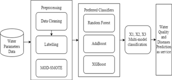
Classification algorithm model approach.

Random Forest

Random forest is one of the popular ensemble techniques to reduce overfitting and increase the generalization of the model. It works by combining multiple decision trees with each decision tree working on a different set of subsets and features and hence the final decision is taken by voting principle³⁷.

According to its definition, Random Forest is a general method combination of classifiers that use L tree-structured base classifiers {h (\(\:X,\:{\theta\:}_{n}\)), N = 1,2,3, …, L}, where \(\:X\) denotes the input data and {\(\:{\theta\:}_{n}\)} is a group of distributed random vectors that are all the same and dependent.

\({\text{p}}={\text{mode~}}\left\{ {{T_1}\left( {\text{y}} \right),{T_2}\left( {\text{y}} \right),{\text{~}}{T_3}\left( {\text{y}} \right),{\text{~}} \ldots ,{T_m}{\text{~}}\left( {\text{y}} \right)} \right\}\)

\({\text{p}}={\text{mode~}}\left\{ {{\text{\varvec{\Sigma}m}}={1_m}{T_m}\left( {\text{y}} \right)} \right\}\)

There are \(\:{T}_{1}\)(y), \(\:{T}_{2}\)(y), \(\:{T}_{3}\)(y), …, \(\:{T}_{m}\)(y) decision trees involved in the prediction process, and p represents the choice that received the majority of votes.

The phrase “random state” is used in RF to control the sample’s unpredictability during training.

AdaBoost

For classification and regression problems, AdaBoost machine learning is used. It works by creating a strong learner from several weak ones. In each iteration of the method, the weak learner is trained on the data, and instances that were mistakenly categorized are given more weight to be classified correctly in the following iteration. In the final model, the weak learners are combined, and their weights are determined by how well they did throughout training. AdaBoost has been used successfully in a variety of areas, such as bioinformatics, text categorization, and face recognition. High precision and the ability to handle complex datasets are two of its most famous qualities.

The AdaBoost algorithm retains a collection of weights across training data and adapts them after each cycle of poor learning to generate a group of learners who are weak at learning. Weights for the training samples that the present poor learner incorrectly classified will rise, but weights for the examples that were correctly classified would decline³⁸.

XGBoost

XGBoost, or extreme gradient boosting, is a popular machine learning method for supervised learning problems. It is a strong and effective algorithm that is increasingly used to create prediction models, especially in contests on websites like Kaggle. The gradient boosting theory, which comprises gradually adding decision trees to an ensemble to improve prediction accuracy, forms the basis of XGBoost. With each repetition, the model becomes better at anticipating the leftover faults from the previous iteration. The model then combines the results of each tree to get a result. Up until the model reaches a set number of trees, or until the performance does not noticeably improve, whichever comes first³⁹.

One of XGBoost/s key features is its capacity to handle missing information and feature selection. It penalizes complex models through a process called “regularization,” which might help prevent overfitting. It may be used for classification and regression applications and supports a variety of loss functions.

XGBoost’s scalability and efficacy are widely known. It is capable of handling enormous datasets with a variety of properties and can operate in parallel on many CPUs and GPUs. Also, it has several optimization techniques, such as the ability to separate continuous features using a histogram-based technique, which might significantly speed up training.

In conclusion, XGBoost is a strong and adaptable machine-learning algorithm that can be applied to a variety of predictive modeling issues. Its popularity in competitions and industrial applications has made it an important tool for data scientists and machine learning practitioners.

Tables 7 and 8 provide a comparison of classification performance before and after using the MOD-SMOTE approach, including key metrics including precision, recall, F-score, and accuracy. Table 7, which depicts classification without MOD-SMOTE, demonstrates inferior performance owing to unbalanced data, resulting in poor detection of minority classes. In comparison, Table 8 indicates that using MOD-SMOTE results in considerable gains across all measures. This is because MOD-SMOTE balances the dataset by creating synthetic examples for the minority class, resulting in higher model accuracy and more trustworthy predictions. This comparison shows how MOD-SMOTE improves the model’s capacity to accurately categorise under-represented cases, resulting in better overall performance.

Figure 8 compares the performance of three classifiers—Random Forest, AdaBoost, and XGBoost—with and without MOD-SMOTE, utilising measures such as precision, recall, F-score, and accuracy. Without MOD-SMOTE, all classifiers have decreased recall and F-scores, with minority class prediction especially difficult owing to data imbalance, while total accuracy may still look good. MOD-SMOTE enhances performance in all parameters, including accuracy, recall, and F-score, suggesting more balanced and accurate categorisation. MOD-SMOTE significantly improves these models’ capacity to accurately categorise both majority and minority classes, suggesting its utility in enhancing classification performance. In comparison, Random Forest has outperformed the other two models.

Comparison of classification performance.

One of the most important reasons why Random Forest outperforms is because it is an ensemble algorithm that reduces variance by combining the results of several decision trees generated at different bootstrap samples of the learning set, thereby providing better overall prediction accuracy. This model does well on a large number of high-dimensional datasets and adequately handles both numerical and categorical variables. Moreover, Random Forest avoids overfitting to some extent because it uses the average of multiple predictions. For this model demonstrates high precision because it captures complications within such a water quality dataset and even deals with imbalanced datasets by resampling techniques that further improve its robustness in the applicatory world. The very fast execution time mentioned in the time-tracking metric in Table 9 is also another feature that highlights the efficiency of rapid, quick predictions.

The graphical representation of Table 9 is depicted in Fig. 9.

Comparison of classification model execution time.

C. TS-SMOTE.

The frequency of the data samples in the dataset should have a natural time interval of measurement. The frequency of the dataset represents the number of observations made before the seasonal pattern repeats. Therefore, to make the dataset suitable for forecasting TS-SMOTE is used as mentioned in Section III.C. The dataset generated from TS-SMOTE is used further in Forecasting in Section IV.D.

D. Forecasting.

LSTM Model

Figure 10 depicts the layout of a Long Short-Term Memory (LSTM) model, showing essential components such as input gates, forget gates, output gates, and memory cells, which work together to capture long-term relationships in sequential data. Recurrent neural network (RNN) architectures like the LSTM model are designed to recognise long-term relationships in sequential data. When typical RNNs attempt to learn long-term dependencies, they often run into the vanishing gradient problem. This solution overcomes this difficulty. The LSTM does this by including a memory cell and many gates that control the information flow. It has proved effective in a number of applications including natural language processing, audio recognition, and time series analysis and is able to capture long-term dependencies. LSTM networks are particularly useful when the data has complex temporal dynamics.

Architecture of LSTM model with its components.

The proposed LSTM model

The structure of the suggested LSTM network is shown in Fig. 11. Each of the four LSTM layers in the prediction model comprises 64 units. To create an improved forecasting model, the network contains two feed-forward layers after the LSTM layers, one with 32 units and one with only one unit.

As a result, the suggested model has almost 144,633 trainable parameters, reducing the time to train the model.

To train the LSTM-based deep neural network, a dataset of time-series was constructed by creating windows of 90 consecutive precipitation values. Each window consisted of 90 rainfall observations, and the corresponding output value was the 91st value in the dataset, representing the subsequent consecutive observation. In total, 92,450 windows of consecutive rainfall measurements were generated for training the LSTM model. A training set and a testing set were created from the dataset at a ratio of 80:20, respectively.

Dataset preparation

The system created a windowed time-series dataset with a window size of 90, consisting of 90 consecutive precipitation values in each window. Each window’s input sequence comprised the first 90 values, and the corresponding output was set as the 91st value. This resulted in a total of 92,450 windows of consecutive rainfall measurements.

Train-test split

The dataset was split into training and testing sets using an 80:20 ratio. Specifically, 80% of the windows (73,960 windows) were allocated for training, while the remaining 20% (18,490 windows) were reserved for testing.

Model architecture

The implemented prediction model featured four LSTM layers, each consisting of 64 units. Following the LSTM layers, the network included two feed-forward layers: one with 32 units and one with a single unit. This architecture was designed to build an optimized forecasting model.

Hyperparameter optimization

Hyperparameter optimization techniques were employed to fine-tune the model’s performance. Specific values were chosen for each hyperparameter during the optimization process. Example hyperparameter values: Number of LSTM Layers: 4, Units per LSTM Layer: 64, Units in the First Feed-Forward Layer: 32, Units in the Second Feed-Forward Layer: 1.

Model compilation

The model was compiled by specifying the necessary components, including the loss function and optimizer. To measure the disparity between the values, the loss function was mean squared error (MSE) was used that were anticipated and those that were actually obtained. With additional default values and a learning rate of 0.001, the Adam optimizer was used.

Model training

The LSTM model was trained using the prepared training data and the specified hyperparameters. The training process involved running 100 epochs to ensure sufficient training iterations without overfitting. A batch size of 32 was chosen to process 32 samples at each iteration before updating the model’s parameters.

Performance evaluation

The model’s performance on the testing set was assessed after the training phase. To measure the precision of the model’s predictions, evaluation measures including mean absolute error (MAE) and root mean square error (RMSE) were used. The model’s performance, including accuracy and validation loss, was carefully analyzed to ensure the best results were achieved.

Hyperparameter tuning

To enhance the performance of the LSTM model, an extensive hyperparameter tuning process was conducted to optimize its configuration further. To effectively explore the hyperparameter space and identify the ideal combination, methods like random search and Bayesian optimization were used. Example hyperparameter tuning using random search: Number of LSTM Layers: randomly selected from^2,4,6 (selected value: 4), Units per LSTM Layer: randomly selected from [32, 64, 128] (selected value: 64), Learning Rate: randomly selected from [0.0001, 0.001, 0.01] (selected value: 0.001), Batch Size: randomly selected from [16, 32, 64] (selected value: 32), Number of Epochs: randomly selected from [50, 100, 150] (selected value: 100), Random search efficiently sampled hyperparameter combinations and evaluated their performance, enabling a more targeted exploration., The combination that yielded the best performance, considering accuracy and validation loss, was selected as the optimized hyperparameters for the LSTM model.

Iterative refinement

To further enhance the model’s performance and address any remaining issues, an iterative refinement process was implemented. Various techniques were applied iteratively to optimize the model’s generalization and prevent overfitting. Example iterative refinement techniques: Regularization: Dropout with a rate of 0.3 was applied to the LSTM layers to improve generalization. Learning Rate Scheduling: If the validation loss did not decrease after 10 epochs, the learning rate was decreased by a factor of 0.01. Early Stopping: To reduce overfitting, training was terminated if the validation loss did not become better after 20 iterations. These refinement techniques were systematically applied, and the model’s performance was assessed at each iteration to determine their impact and select the most effective settings.

By incorporating these enhancements to the Hyperparameter Tuning and Iterative Refinement steps, the LSTM model’s training process was further optimized. The hyperparameters were fine-tuned through techniques like random search, allowing for a more comprehensive exploration of the hyperparameter space. Iterative refinement techniques, such as regularization, learning rate scheduling, and early stopping, were applied to optimize the model’s generalization and achieve the best accuracy and minimum validation loss.

Evaluation metric

In forecasting research and analysis, various evaluation metrics are used to assess the accuracy and performance of forecasted values. Among the commonly used metrics are the Root Mean Squared Error (RMSE), which measures the average magnitude of the forecast errors, the Mean Absolute Error (MAE), which quantifies the average absolute difference between forecasted and actual values, and the R-squared (R2) value, which shows the percentage of the variance in actual values that can be explained by the forecasted values. Additionally, the Mean Forecast Error (MFE) captures the average difference between forecasted and actual values, while the Mean Percentage Error (MPE) and Mean Absolute Percentage Error (MAPE) provide insight into the average percentage difference between forecasts and actual values. Lastly, the Directional Accuracy (DA) metric evaluates the proportion of correct directional forecasts.

Table 10 compares the assessment metrics of a normal LSTM model with the proposed LSTM model for predicting the pH parameter, including MAE, RMSE, MAPE, and R² and graphical represented in Fig. 12.

Evaluation metrics: LSTM vs. proposed LSTM.

The line graph compares the performance of the LSTM and Proposed LSTM models using various evaluation metrics. The Proposed LSTM model outperforms the LSTM model across most metrics, showing lower errors (MAE, RMSE) and higher accuracy (R2, DA). The above Actual value [7.642, 7.881, 7.552, 7.693, 7.453, 7.894, 7.712, 7.644, 7.568, 7.814, 7.836, 7.678, 7.725, 7.979, 7.538, 7.937, 7.554, 7.399, 7.642, 7.835] and Forecasted value are [7.699, 7.358, 7.918, 7.548, 7.648, 7.271, 7.876, 7.481, 7.736, 7.609, 7.842, 7.426, 7.998, 7.679, 7.563, 7.953, 7.514, 7.378, 7.784, 7.625]. The analysis conducted helps us gain insights into Metabolic Alkalosis, a medical condition characterized by an elevation in the pH level of the body. Metabolic Alkalosis can occur due to various factors but based on the given pH parameter range of 7–8.5 for 2 to 3 weeks, it is concluded that this specific pH range alone cannot be the cause of Metabolic Alkalosis. Table 11 shows the assessment metrics for the proposed model’s predicted fluoride and pH parameters and graphically represented in Fig. 13.

Evaluation metrics for fluorides and PH: LSTM vs. proposed LSTM.

The analysis focused on the Fluorides and pH parameters, with a maximum permissible range of 1.5 for Fluorides and 6.5–8.5 for pH if exceed 108–350 Weeks then it can cause Dental Problems. The evaluation metrics indicate the performance of LSTM and Proposed LSTM models in predicting the values for these parameters. The Proposed LSTM model generally shows better performance across most metrics compared to LSTM, with lower MAE, RMSE, and MPE values and higher R2 and DA values. This suggests that the Proposed LSTM model provides improved accuracy and prediction capability for both Fluorides and pH parameters. With reference to Table 12. The analysis focused on two parameters: Fluorides and pH. The evaluation metrics were used to assess the performance of the LSTM and Proposed LSTM models in predicting these parameters. For the Fluorides parameter, the Proposed LSTM model outperformed the LSTM model in terms of MAE, RMSE, R2, MFE, MPE, MAPE, and DA. The Proposed LSTM model achieved lower error values (MAE and RMSE), higher R2 indicating better explanatory power, and higher DA representing improved directional accuracy. These results suggest that the Proposed LSTM model provides more accurate and reliable forecasts for Fluorides.

Similarly, for the pH parameter, the Proposed LSTM model exhibited superior performance compared to the LSTM model across all evaluation metrics. It achieved lower MAE and RMSE values, higher R2 indicating better explanatory ability, and higher DA suggesting improved directional forecasting accuracy. The Proposed LSTM model’s forecasts for pH were more accurate and aligned closely with the actual values. Based on the analysis of the Fluorides and pH parameters, it can be concluded that the Proposed LSTM model demonstrates better predictive capabilities than the LSTM model. The proposed model provides more accurate forecasts for both Fluorides and pH, making it a valuable tool in forecasting these parameters for various applications such as water quality monitoring and healthcare. It’s worth noting that the analysis considered the permissible ranges for Fluorides and pH. For Fluorides, a maximum permissible range of 1.5 was considered, while for pH, the range of 6.5–8.5 was assessed. It was observed that the forecasted values did not exceed these ranges, indicating that the forecasted values are within acceptable limits and not likely to cause dental problems or metabolic alkalosis.

These factors could show the improvements of future predictions. First, extend the data set to include extrinsic parameters such as temperature, humidity, or human activity data, which would give a deeper insight into environmental factors that may affect water quality. Later refinements in the procedure for the optimization of hyperparameters could be more advanced techniques like Bayesian optimization, to further improve accuracy. The ensemble learning approach that combines LSTMs with other models such as Random Forests or Gradient Boosting improves the robustness of the predictions. Lastly, the usual ongoing refinement of regularization techniques and use of a more dynamic learning rate schedule during training may avoid overfitting and improve the generalization of the model towards future use on diverse and changing conditions.

Overall, the Proposed LSTM model demonstrates promising performance and can be relied upon for accurate forecasting of Fluorides and pH parameters, contributing to effective decision-making and better understanding of water quality and health-related implications.