
Optimizing healthcare big data performance through regional computing

The healthcare system becomes more efficient as more data from IOMT is integrated into the collective network. Uploading data from every device to cloud servers is essential; however, each medical device may generate up to a terabyte of data per day, which is beyond the capacity of existing systems to transport, process, and store efficiently. As illustrated in Fig. 4, the proposed system seeks to process and store this medical big data closer to healthcare infrastructure to reduce latency and cost. The data is then transferred to the cloud during off-peak hours, ensuring minimal network load, as peak hours often lead to congestion, whereas off-peak periods are typically underutilized. The proposed model look at the performance (network and data-center), energy and cost model. The remaining part of this section, covers this in detail.

Proposed structure of regional computing for healthcare data-driven applications.
Delay model
The delay model is structured into three layers: the IOMT, responsible for managing all healthcare devices; regional computing, which handles the processing of healthcare big data near the devices; and cloud computing, which ensures permanent data storage and supports large-scale analysis. The following sections detail the operation of this methodology.
Internet of medical things (IoMT)
The IOMT layer includes the medical devices, and sensors. Data from these devices (\(w = \{w_{1}, w_{2}, w_{3}, \ldots , w_{m}\}\)) , such as wearable sensors, implantable medical devices, or external monitoring systems (\(d = \{d_{1}, d_{2}, d_{3}, \ldots , d_{n}\}\)), is transmitted to gateways through personal or local area networks, which act as collectors and edge for transferring data to the regional servers for processing and analysis. The medical sensors, such as Electrocardiogram (ECG) monitors, pulse oximeters, and glucose sensors, collect real-time health data, while gateways help ensure efficient data transmission to minimize latency and support immediate healthcare needs. This communication involves various delays during the data transmission process. These delays include transmission delay, propagation delay, processing delay, and queuing delay, each contributing to the overall time required for the data to reach its destination.
Most of the sensors are wirelessly connected to the gateway through a personal area network and wirelessly transmit the data. Transmission delay (\(T_{\text {tran}}\)) accounts for the time taken to transmit the data from the IOMT device (d) to the gateway. It is determined by factors including data (\(Wl\)), channel bandwidth (\(B\)), signal-to-noise ratio (\(SNR\)), modulation efficiency (\(M\)), and error rate (\(E\)). This relationship is expressed as:
$$\begin{aligned} T_{\text {tran}} = \frac{Wl \times M \times \text {SNR}}{B \times E} \end{aligned}$$
(1)
The propagation delay (\(T_{\text {prop}}\)) represents the time taken for the data to travel through the wireless medium. It depends on the distance (\(d\)) between the IOMT device and the gateway and the transmission speed (\(v\)) in the medium:
$$\begin{aligned} T_{\text {prop}} = \frac{d_{gateway}}{v} \end{aligned}$$
(2)
The processing delay (\(T_{\text {proc}}\)) reflects the time taken for the gateway to process the received data. It is determined by the data workload (\(Wl\)) and the processing rate of the gateway (\(R_{\text {proc}}\)):
$$\begin{aligned} T_{\text {proc}} = \frac{Wl}{Pr_{\text {gateway}}} \end{aligned}$$
(3)
Finally, the queuing delay (\(T_{\text {que}}\)) indicates the time the data spends in the gateway’s queue before being processed. This depends on the workload (\(Wl\)), packet arrival rate (\(\lambda\)), and the processing capacity (\(\mu\)) of the gateway:
$$\begin{aligned} T_{\text {que}} = \frac{Wl \times \lambda }{\mu } \end{aligned}$$
(4)
where \(Wl = \sum _{i=1}^{n} d_i\), workload generated by 1 to n medical devices.
Combining all these components, the total delay for data communication from IOMT devices to the gateway through the PAN or LAN can be expressed as:
$$\begin{aligned} T_{\text {Gatway}} = \frac{Wl \times M \times \text {SNR}}{B \times E} + \frac{d}{v} + \frac{Wl}{Pr_{\text {gateway}}} + \frac{Wl \times \lambda }{\mu } \end{aligned}$$
(5)
This Eq. (5) provides a comprehensive way to calculate the total delay in an IOMT layer, taking into account various factors such as data transmission, propagation, processing, and queuing delays.
Regional computing
To optimize network efficiency, the HBD generated by IOMT devices is temporarily stored on regional servers during peak hours and transmitted to the cloud during off-peak periods. This approach alleviates congestion on public networks and minimizes latency.
The regional layer consists of servers dedicated to processing and storing data from healthcare devices within a specific geographical area. These servers function as regional servers, aggregating information from various healthcare devices operating in their domain. Each device transmits data to the regional servers, which encompass parameters such as patient monitoring data, device status, environmental conditions, and other relevant information regarding health and safety.
This data from gateways to the regional servers is transmitted through fibre optic or other fast transmission medium. The transmission delay (\(T_{\text {tran}}\)) in this context depends on the data size (\(Wl\)), and the speed (\(v\)). The transmission delay can be expressed as:
$$\begin{aligned} T_{\text {tran}} = \frac{Wl}{v} \end{aligned}$$
(6)
The propagation, queuing and processing delay are the same as calculated for IOMT layer.
$$\begin{aligned} T_{\text {Regional}} = \frac{d}{v} + \frac{Wl}{Pr_{\text {regional}}} + \frac{L \times \lambda }{\mu } \end{aligned}$$
(7)
The Eqs. 5 and 7 demonstrate that the delay is primarily influenced by the total workload and the transmission distance. Therefore, by reducing both the network workload and the distance, the overall delay experienced by HBD can be significantly minimized.
The major part of the workload in this IOMT architecture is processed by regional computing units, significantly reducing the burden on central cloud infrastructure and, consequently, minimizing network congestion. By handling data closer to the source, regional computing limits the amount of traffic transmitted over the mainstream network, thus reducing the total traffic, \(Wl_{total}\), on the network. As a result, this approach helps maintain an optimal balance between workload and available bandwidth, \(B_{avail}\), as illustrated by the following congestion probability equation:
$$\begin{aligned} Con_{Prob} \approx \frac{Wl_{total}}{B_{avail}} \end{aligned}$$
here, \(Con_{Prob}\) denotes the probability of congestion, which is directly proportional to the total network traffic and inversely proportional to the available bandwidth. Since regional computing handles the bulk of the processing locally, \(Wl_{total}\) decreases, effectively lowering the likelihood of congestion.
Regional computing’s decentralized approach, by reducing the volume of data sent to the cloud, optimizes bandwidth usage and mitigates network congestion risks, ensuring faster data processing and enhanced real-time IOMT services. This architecture not only improves efficiency but also supports scalable healthcare solutions as IOMT devices proliferate.
Cloud computing
The regional layer manages real-time medical data from IOMT devices, while the cloud layer operates as a powerful backend that enhances data processing and storage capabilities. The regional layer relies on the cloud for extensive computing resources, transferring medical big data to the cloud during off-peak hours to utilize its advanced capabilities for comprehensive analysis and share the data globally for research and diagnostic purposes.
In contrast to the regional layer, the cloud hosts a vast amount of HBD generated from worldwide medical centres. It functions as a centralized repository for processing and storing this extensive dataset.
$$\begin{aligned} T_{\text {cloud}} = \frac{Wl}{Pr_{\text {cloud}}} \end{aligned}$$
(8)
Equation (8) illustrates the processing time (\(T_{\text {cloud}}\)) required to collectively analyze all medical workloads at cloud servers. Here, \(T_{\text {cloud}}\) represents the processing time, \(Wl\) is the total medical workload to be processed, and \(Pr_{cloud}\) is the processing rate of the cloud servers, denoting the volume of data processed per unit of time.
The total medical big data workload (\(Wl\)) is calculated as the summation of data produced by each IOMT device (\(d_i\)) from 1 to \(n\), as shown in Eq. (9):
$$\begin{aligned} Wl = \sum _{i=1}^{n} d_i \end{aligned}$$
(9)
Similarly, the propagation delay (\(T_{\text {prop}}\)) represents the time taken for the data to travel through the network. It depends on the distance (\(d_{cloud}\)) between the IOMT device and the cloud servers and the transmission speed (\(v\)) in the medium:
$$\begin{aligned} T_{\text {prop}} = \frac{d_{cloud}}{v} \end{aligned}$$
(10)
Analysis of Eqs. (9) and (10) indicates that the round-trip to the cloud incurs more delay than anticipated. This increased delay is primarily due to the cloud’s necessity to process substantial volumes of medical big data (\(Wl\)) and its distance (d). Additionally, propagation and queuing delays escalate in correlation with the growing workload and distance.
The cloud plays a crucial role in analyzing Medical Big Data (MBD) to derive insights into patient health, treatment effectiveness, and device performance. These insights improve healthcare delivery, providing real-time updates to healthcare providers and enhancing patient outcomes. Additionally, the cloud strengthens safety and security measures by detecting anomalies, identifying risks, and optimizing healthcare practices.
Energy model
In healthcare big data, energy consumption plays a critical role, especially when handling the vast amount of data generated by medical devices. Similar to delay, energy consumption is also impacted by the distance between devices. The energy consumption in HBD communication can be computed as:
$$\begin{aligned} \mathscr {E}_{\text {tran}} = \sum _{i=1}^{n} \left( \mathscr {E}_{\text {tran}}^{\text {sensor}}(i) + \mathscr {E}_{\text {tran}}^{\text {regional}}(i) \right) \end{aligned}$$
(11)
here, \(\mathscr {E}_{\text {tran}}^{\text {sensor}}(i)\) represents the energy used for data transmission from medical sensor \(i\) to the gateway, while \(\mathscr {E}_{\text {tran}}^{\text {regional}}(i)\) refers to the energy utilized for transferring data from the gateway to regional servers.
Where
$$\begin{aligned} \mathscr {E}_{\text {tran}}^{\text {sensor}}(i)\approx {Dis_{i, \text {gateway}} \cdot P_{i}^{\text {sensor}}}\cdot {{T_{i, \text {gateway}}}} \end{aligned}$$
(12)
and
$$\begin{aligned} \mathscr {E}_{\text {tran}}^{\text {regional}}(i) \approx {Dis_{\text {gateway}, \text {regional}} \cdot P_{\text {gateway}}^{\text {regional}}}\cdot {{T_{\text {gateway}, \text {regional}}}} \end{aligned}$$
(13)
In these equations, \(Dis_{i, \text {gateway}}\) denotes the distance between medical sensor \(i\) and the gateway, \(P_{i}^{\text {sensor}}\) represents the power consumption for data transmission by sensor \(i\), and \(T_{i, \text {gateway}}\) is the time taken for the data to reach the gateway. Similarly, \(Dis_{\text {gateway}, \text {regional}}\) represents the distance from the gateway to the regional server, \(P_{\text {gateway}}^{\text {regional}}\) is the power consumption for data transmission, and \(T_{\text {gateway}, \text {regional}}\) represents the transmission time from the gateway to the regional servers.
These equations demonstrate that energy consumption increases with the distance involved in data transmission, both from sensors to gateways and from gateways to regional servers through network.
$$\begin{aligned} \mathscr {E}_{\text {other}} = \mathscr {E}_{\text {pro}} + \mathscr {E}_{\text {stor}} + \mathscr {E}_{\text {cool}} + k \end{aligned}$$
(14)
Similarly, \(\mathscr {E}_{\text {other}}\) encompasses the energy used for other operations such as data processing (\(\mathscr {E}_{\text {pro}}\)), storage (\(\mathscr {E}_{\text {stor}}\)), and cooling (\(\mathscr {E}_{\text {cool}}\)) in medical data centers.
The total energy consumption for the IOMT system is calculated as:
$$\begin{aligned} \mathscr {E}_{\text {total}} = \mathscr {E}_{\text {tran}} + \mathscr {E}_{\text {other}} \end{aligned}$$
(15)
where \(\mathscr {E}_{\text {total}}\) represents the overall energy consumption, while \(\mathscr {E}_{\text {tran}}\) denotes the total energy consumed during data offloading from IOMT devices.
It is important to note that:
$$\begin{aligned} Cost_{\text {oper}} \propto \mathscr {E} \end{aligned}$$
(16)
There is a direct relationship between energy consumption (\(\mathscr {E}\)) and operational costs (\(Cost_{\text {oper}}\)). As energy consumption increases, the operational costs of managing and processing medical big data also rise.
The equations above indicate that energy consumption escalates as the distance between IOMT sensors and regional servers increases. Moreover, the increasing workload can congest network channels and computing processors, generating additional heat and further energy consumption (as shown in Eq. 16). Consequently, this model shows that energy consumption for cloud-based processing of medical big data is significantly higher. However, when workloads are processed by regional servers, energy requirements are reduced, making regional computing a more energy-efficient solution for HBD.
Cost model
In prior sections, we examined how delay, congestion, and energy consumption escalate with the increasing distance between medical devices and processing units within the IOMT framework. This section highlights the cost dynamics associated with these parameters for HBD. The total cost can be expressed using the following equation:
$$\begin{aligned} Cost_{t} = Cost_{tr} + Cost_{p} + Cost_{pr} + Cost_{col} \end{aligned}$$
(17)
where \(Cost_{t}\) signifies the total cost, \(Cost_{tr}\) denotes the transmission cost, \(Cost_{p}\) is the propagation cost, \(Cost_{pr}\) refers to the processing cost, and \(Cost_{col}\) accounts for the cooling cost associated with medical data storage and processing facilities.
The transmission cost, \(Cost_{tr}\), encompasses two components: the expense related to transmitting data from IOMT devices to central data aggregation points and the cost incurred from these aggregation points to regional computing servers.
For the transmission from IOMT devices to gateway, the cost can be formulated as:
$$\begin{aligned} \begin{aligned} C_{\text {trn, gateway}}&= \sum _{i=1}^{n} \sum _{j=1}^{m} \left( C_{\text {rate, dev}} \cdot L_{i,\text {gateway}} w_j + \right. \\&\quad \left. C_{\text {time, dev}} \cdot T_{i,\text {gateway}} + C_{\text {energy, dev}} \cdot E_{i,\text {agg}} + \right. \\&\quad \left. C_{\text {bandwidth, dev}} \cdot B_{i,\text {gateway}} + C_{\text {fixed, dev}} \right) \end{aligned} \end{aligned}$$
(18)
In this formula, \(n\) represents the number of IOMT devices, and \(m\) denotes the number of workload tasks generated by these devices. \(C_{\text {rate, dev}}\) signifies the cost per unit of data transmitted, with \(L_{i,\text {gateway}} w_j\) indicating the data amount from IOMT device \(i\) for workload \(j\). \(C_{\text {time, dev}}\) refers to the cost per unit of time for this transmission, while \(T_{i,\text {gateway}}\) represents the required transmission time. \(C_{\text {energy, dev}}\) denotes the cost per unit of energy consumed, with \(E_{i,\text {gateway}}\) representing the energy utilized in the transmission from IOMT devices to data aggregation points. Additionally, \(C_{\text {bandwidth, dev}}\) indicates the cost per unit of bandwidth used, and \(B_{i,\text {gateway}}\) signifies the bandwidth utilized. \(C_{\text {fixed, dev}}\) is the fixed cost associated with each transmission event from IOMT devices.
For the transmission from gateway to regional computing servers, the cost can be formulated as:
$$\begin{aligned} \begin{aligned} C_{\text {trn, rc}}&= \sum _{i=1}^{n} \sum _{j=1}^{m} \left( C_{\text {rate, gateway}} \cdot l_{\text {gateway},\text {rc}} w_j + \right. \\&\quad \left. C_{\text {time, gateway}} \cdot T_{\text {gateway},\text {rc}} + C_{\text {energy, gateway}} \cdot E_{\text {gateway},\text {rc}} + \right. \\&\quad \left. C_{\text {B, gateway}} \cdot B_{\text {gateway},\text {rc}} + C_{\text {fixed, gateway}} \right) \end{aligned} \end{aligned}$$
(19)
In this formula, \(C_{\text {rate, gateway}}\) signifies the cost per unit of data transmitted from gateway, with \(l_{\text {gateway},\text {rc}} w_j\) representing the data amount for workload \(j\). The cost per unit of time for this transmission is \(C_{\text {time, gateway}}\), with \(T_{\text {gateway},\text {rc}}\) indicating the time taken. \(C_{\text {energy, gateway}}\) denotes the cost per unit of energy consumed during this transmission, while \(E_{\text {gateway},\text {rc}}\) represents the energy used in the transmission from the gateway to regional computing servers. \(C_{\text {B, gateway}}\) is the cost per unit of bandwidth utilized, and \(B_{\text {gateway},\text {rc}}\) signifies the bandwidth utilized. Lastly, \(C_{\text {fixed, gateway}}\) is the fixed cost associated with each transmission event from aggregation points.
The total transmission cost can be calculated as:
$$\begin{aligned} C_{\text {trn}} = C_{\text {trn, gateway}} + C_{\text {trn, rc}} \end{aligned}$$
(20)
The propagation cost, \(Cost_{p}\), is determined based on the distances involved and is expressed as:
$$\begin{aligned} C_{\text {prop}} = \sum _{i=1}^{n} \left( C_{\text {dis, dev}} \cdot Dis_{i,\text {gateway}} + C_{\text {dis, gateway}} \cdot Dis_{\text {gateway},\text {rc}} \right) \end{aligned}$$
(21)
In this equation, \(C_{\text {dis, dev}}\) is the cost per unit of distance for IOMT device-to-aggregation point transmission, while \(Dis_{i,\text {gateway}}\) is the distance from IOMT device \(i\) to the aggregation point. \(C_{\text {dis, gateway}}\) signifies the cost per unit of distance for aggregation-to-regional computing transmission, with \(Dis_{\text {gateway},\text {rc}}\) representing the distance involved in this stage.
The processing cost \(Cost_{pr}\) is computed as:
$$\begin{aligned} C_{\text {prc}} = \sum _{i=1}^{n} \sum _{j=1}^{m} \left( C_{\text {uprc}} \cdot T_{\text {prc}_{i,j}} \right) \end{aligned}$$
(22)
here, \(T_{\text {prc}_{i,j}}\) denotes the processing time for data from IOMT device \(i\) and workload \(j\), and \(C_{\text {uprc}}\) signifies the processing time cost per unit.
This comprehensive cost model encompasses the expenses associated with transmitting data from IOMT devices to gateway and then to the regional computing servers, as well as the propagation and processing costs involved in handling HBD.
The cost model equations demonstrate the significant influence of distance on transmission and propagation costs, along with processing time on overall expenses (as illustrated in Eqs. 18, 19, and 22). Due to the increased distances involved in data transmission, cloud computing generally incurs higher costs. In contrast, regional computing optimizes costs by minimizing transmission distances and enhancing processing efficiencies, rendering it a more cost-effective approach for managing HBD.
Algorithm
The Algorithm 1 is designed to handle the large-scale data generated by IOMT devices, including wearables, medical imaging systems, remote monitoring, and emergency response systems. The data generated from these sources \(D = \{d_{1}, d_{2}, d_{3}, \ldots , d_{n}\}\), and their associated workloads \(w = \{w_{1}, w_{2}, w_{3}, \ldots , w_{m}\}\), are processed through a tiered system, which leverages Edge Computing (EC) (Gateway) for immediate, real-time needs, RC for intermediate tasks, and Cloud Computing (CC) for intensive processing.
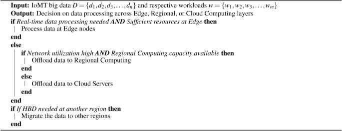
IoMT big data processing and offloading.
The IOMT algorithm functions by efficiently distributing data processing across multiple layers (Edge, Regional, and Cloud Computing) based on the needs of the healthcare applications and the current network conditions. Initially, as shown in Fig. 5, data generated by IOMT devices, such as wearables or emergency systems, is checked to determine if it requires immediate processing. If the data is time-sensitive and gateway resources are available, the algorithm processes it locally. This ensures minimal delay and provides real-time analytics, which is essential for critical healthcare applications like patient monitoring or urgent diagnoses.

Flowchart for healthcare big data.
When network utilization is high and edge resources are insufficient, the algorithm considers offloading the data to RC. If the regional servers have available capacity, the data is processed at this intermediate layer. This step helps in balancing resource utilization while minimizing the dependency on external cloud services.
In situations where neither EC nor RC is viable, or if the data processing tasks are particularly resource-intensive, such as those involving medical imaging analysis, the algorithm shifts the workload to Cloud Computing. This ensures that more computationally demanding tasks are handled efficiently, even if it increases the dependency on centralized cloud resources. For critical or urgent medical tasks where real-time data analysis or rapid migration to other regions is necessary, the algorithm gives priority to cloud processing. Additionally, it supports the migration of critical data to other regions for immediate analysis and decision-making. By following this tiered processing approach, the algorithm ensures that HBD is managed efficiently, providing real-time patient care while balancing network traffic and optimizing resource allocation. This structure helps healthcare systems address the growing demands of data-intensive medical applications, ensuring timely insights and interventions.
link


![Average Cost of Medical School [2025]: Yearly + Total Costs](https://educationdata.org/wp-content/uploads/2025/09/page-1.png "Average Cost of Medical School [2025]: Yearly + Total Costs")
