Prediction analysis of human brucellosis cases in Ili Kazakh Autonomous Prefecture Xinjiang China based on time series

Data sources

This study has received formal approval from the Ili Kazakh Autonomous Prefecture Center for Disease Control and Prevention. The data used in the research come from the county-level administrative units of the Ili Kazakh Autonomous Prefecture, covering the monthly reported cases of human brucellosis from January 2010 to September 2023. The data from January 2010 to January 2021 are used as the training set for model training, while the data from February 2021 to September 2023 are used as the prediction set to evaluate the predictive performance of the models. The diagnostic criteria for human brucellosis follow the health industry standard of the People’s Republic of China, “Brucellosis Diagnosis” (WS269-2019).

Based on China’s prevention and control policies for COVID-19, the time series is divided into the COVID-19 pandemic period and the non-COVID-19 period. This division starts in January 2020, when China first issued control measures for COVID-19, and ends in January 2023, when the Chinese government announced the adjustment of COVID-19 management from “Class B, Category A” to “Class B, Category B”. During this specific period, it is coded as “1”, while the remaining periods are coded as “0”, representing either the absence of the pandemic or the “Class B, Category B” period. Subsequently, this period classification is introduced as a new variable into the optimal model to once again predict the number of human brucellosis cases.

SARIMA model

The incidence characteristics of human brucellosis are characterized by long-term trends, periodicity, and seasonality. ARIMA (Autoregressive Integrated Moving Average model) is a well-established model widely used in time series analysis, highly regarded for its long history of application and excellent performance. Its general form is ARIMA (p, d, q), where p represents the autoregressive order (AR), d represents the differencing order, and q represents the moving average order (MA). However, when time series data exhibits pronounced seasonal patterns, the traditional ARIMA model becomes insufficient. To address this issue, the SARIMA (Seasonal Autoregressive Integrated Moving Average model) was introduced, with its general form being SARIMA (p, d, q) (P, D, Q)s. This model, (p, d, q) handles non-seasonal information. In contrast (P, D, Q) handles seasonal information, where P represents the seasonal autoregressive order (SAR), D represents the seasonal differencing order, Q represents the seasonal moving average order (SMA), and S represents the seasonal period length. By incorporating seasonal components, the SARIMA model can better capture and predict time series data with distinct seasonal characteristics.

In order to deeply understand the characteristics and patterns of the data and to more accurately establish and apply the SARIMA model for future numerical predictions, we first used the STL(Seasonal and Trend decomposition using Loess) method^36,37 to decompose the time series data of human brucellosis. The STL method includes two types of decomposition: additive model decomposition and multiplicative model decomposition. In the multiplicative model decomposition, a logarithmic or Box-Cox transformation of the original series is required. In this study, we chose the additive model decomposition, whose mathematical relationship is expressed as follows:

where \(\textY_\textt\) represents the actual observed value of human brucellosis at time \(\textt\), this value can be decomposed into long-term trend information \(\textT_\textt\), seasonal trend information \(\textS_\textt\), and random fluctuation information \(\textR_\textt\). To ensure the stability of the time series, based on the Autocorrelation Function (ACF) and Partial Autocorrelation Function (PACF), an Augmented Dickey-Fuller (ADF) test is employed to determine whether the entire time series is stationary. If the time series is stationary, no pre-processing is required; otherwise, preprocessing is necessary. In addition, with the assistance of grid search, we can select the optimal combination of model parameters (p, d, q, P, D, Q) according to the Akaike Information Criterion (AIC). Finally, the Ljung-Box (LB) test is used to perform a white noise test on the residuals of the model to ensure that the predictive results of the model are highly accurate.

XGBoost model

XGBoost is an additive model based on the idea of boosting ensemble, first proposed by Tianqi Chen et al³⁸ in 2016. After continuous research and improvement by many scientists, it has become a widely used model in multiple fields. The core concept of the XGBoost model is to achieve the best fit of the data by constructing a combination of multiple predictive functions and assigning weights to each function. The model uses the second-order Taylor expansion as the loss function, effectively addressing the complexity of calculating derivatives for some first-order loss functions. Additionally, XGBoost introduces a regularization term in the loss function, which helps prevent overfitting and improves the generalization ability of the model. The objective function of the XGBoost model is as follows:

where \(\textn\) represents the total number of samples,\(x_i\) denotes the i-th sample, \(f_t(x_i)\) represents the prediction for the i-th sample,\(y_i\) signifies the observed value,\(y_i^(\textt-1)\) indicates the prediction for the i-th sample \(x_i\) on the (t-1)-th tree,\(\Omega (f_t)\) represents the complexity of the t-th tree,\(\textL\) denotes the loss function used to measure the discrepancy between predictions and actual values, and is also used for the output of new trees.γ\(\textT\) is the L1 regularization term aimed at reducing model complexity, while \(\frac12\uplambda \sum_\textj=1^\textT\upomega _\textj^2\) is the L2 regularization term used to smooth parameters and prevent overfitting.\(\textT\) indicates the number of leaves in the decision tree, and \(\upomega\) represents the weight parameters for each leaf node. To ensure the reliability of the model, we use grid search to determine specific hyperparameters, including learning rate, number of estimators, maximum depth, minimum child node weight, gamma, subsample rate, column sample rate, L1 regularization term, and L2 regularization term. Additionally, we employ GridSearchCV for grid searching parameters, with cross-validation utilizing the TimeSeriesSplit from the machine learning library sklearn. TimeSeriesSplit is designed specifically for cross-validation of time series data. It ensures that future data is not used to predict past events during model training, thereby preventing data leakage—the parameter n_splits = 5, indicating a fivefold cross-validation. By manually adjusting the time lag and determining the final value, we adjust as many model parameters as possible to enhance predictive performance and reduce loss bias, enabling the XGBoost model to effectively capture complex patterns in the data.

LSTM model

LSTM networks are a special type of recurrent neural network that can efficiently handle and predict time series data. The structure of an LSTM model consists of four parts: an input layer, LSTM layer, a fully connected layer, and an output layer. Before model training, data is usually normalized for pre-processing to reduce the differences between data points and accelerate the model’s convergence. In this study, the maximum-minimum normalization method was employed. This method scales the data to the range of [-1,1], enhancing the model’s robustness and training efficiency. The formula for this normalization is as follows:

After determining the strategy for data normalization, it is necessary to adjust the hyperparameters of the model, including the learning rate, the number of LSTM layers, the number of neurons in the fully connected layer, and the optimizer, among others. These require careful tuning because these parameters have a crucial impact on the performance of the model. In addition, we have also implemented Dropout to prevent overfitting of the LSTM model. However, the complexity of the model is not always better. An overly complex model may lead to a decrease in generalization ability, meaning the model performs poorly on unseen data. Conversely, an overly simple model may struggle to converge, leading to unstable training and failing to achieve ideal prediction results. Therefore, parameter adjustment requires repeated trials and optimization to ensure that the model maintains good performance while also possessing sufficient generalization ability.

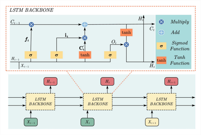
During the training process of a model, selecting the appropriate activation function and loss function is crucial. This study employed the gradient descent algorithm for training the model, using historical data from previous years to train the model to predict future trends in the data. The mathematical expression of the LSTM model is as follows, with its structural diagram shown in Fig. 1

LSTM model structure diagram.

In each layer function of a neural network, there are two crucial attributes: the weight vector and the bias b. These parameters together determine the output of the neural network. The activation function represents each component of the input vector i and denotes the time.

Evaluation and comparison of models

In evaluating the model’s prediction results, we used four metrics: Mean Absolute Error (MAE), Symmetric Mean Absolute Percentage Error (SMAPE), Root Mean Square Error (RMSE), and Coefficient of Determination (R2). Among these, the smaller values of MAE, SMAPE, and RMSE indicate that the model’s prediction results are more accurate. Conversely, the closer the value of R2 is to 1, the better the model’s fitting effect. The definitions of these metrics are as follows:

Data analysis

The Python language as well as relevant third-party libraries were used for writ the model. In this study, the statistical significance level was set at α = 0.05.