Predictive analysis of the number of human brucellosis cases in Xinjiang, China

Drawing the distribution graph (Fig. 1) of the average annual incidence of human brucellosis in China from 2014 to 2017. From which we can see that the incidence of human brucellosis in Xinjiang was higher than that of most provinces. From January 2008 to June 2020, 51,182 cases of human brucellosis were reported in Xinjiang, and the number of reported cases in this period was shown in Fig. 2. From Fig. 2, it could be seen that the time series of human brucellosis cases was obviously seasonal. From May to August of each year, it was the high incidence period of this disease. From 2008 to 2015, the number of human brucellosis cases showed an upward trend. After that, under the vigorous prevention and control of the government and Centers for Disease Control and Prevention in Xinjiang, the number of the brucellosis patients decreased year by year. In February last year, in the case of strict prevention of COVID-19, the incidence of this disease had also been greatly controlled.

The time series of monthly reported cases of human brucellosis in Xinjiang from January 2008 to June 2020.

The prediction analysis of SARIMA model

The SARIMA model is based on stationary data. Firstly, we used Augmented Dickey Fuller’s test (ADF) to test the stationarity of the data. The p-value of the test was 0.56, which indicated that the data was not stationary. Because the data had obvious seasonality (s = 12), we did seasonal differencing to make the data stationary. After the seasonal differencing, the p-value of the ADF test is less than 0.05, and transformed time series appeared to be stationary (see Fig. 3), indicating that the data has been stationary (d = 0, D = 1). Draw the ACF and PACF graphs (see Fig. 4) of the stationary data to help us determining these values of possible p, q, P, and Q. Based on the analysis of Fig. 4, we found that the autocorrelation coefficients were trailing, therefore, we gave q = 0, Q = 1 or 2. For the value of p, we tried taking 1, 2, 4, 5, 6, and 7, respectively. For the value of P, we took 1. Then, the parameters of SARIMA(p,0,0)(P, 1, Q)₁₂ models with different combination of p, P, and Q were tested, and the AIC and SC values of these models were calculated. Finally, only six models (SARIMA(1,0,0)(0,1,0)₁₂, SARIMA((1,4,7),0,0)(0,1,0)₁₂, SARIMA((1,5,7),0,0)(0,1,0)₁₂,SARIMA((1,4,5),0,0)(0,1,2)₁₂,SARIMA((1,4,7),0,0)(0,1,2)₁₂,and SARIMA((1,4,5,7),0,0)(0,1,2)₁₂) passed all parameter tests, as shown in Table 2. Of these six models, model 6 had the smallest AIC and the largest R², so it was the model with the best fitting ability. The expression of model 6 was SARIMA((1,4,5,7),0,0)(0,1,2)₁₂. In order to examine the residuals of the SARIMA((1,4,5,7),0,0)(0,1,2)₁₂ model, we drew the ACF and PACF plots of the model residuals (see Fig. 5). It could be seen from Fig. 5 that the autocorrelation and partial correlation coefficients of the residuals were basically within twice the standard deviation, indicating that the residuals were basically white noise, and the SARIMA((1,4,5,7),0,0)(0,1,2)₁₂ model extracted the information of the original data well and had good performance. Therefore, the SARIMA((1,4,5,7),0,0)(0,1,2)₁₂ model could be used to predict the number of reported cases of human brucellosis in Xinjiang.

Plot of time series after differencing.

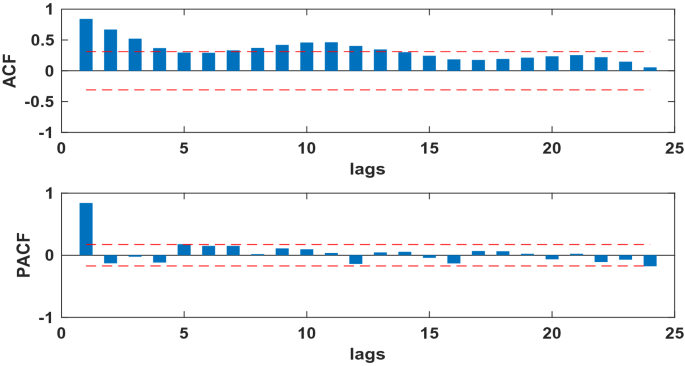
The ACF and PACF of time series after differencing of human brucellosis cases in Xinjiang.

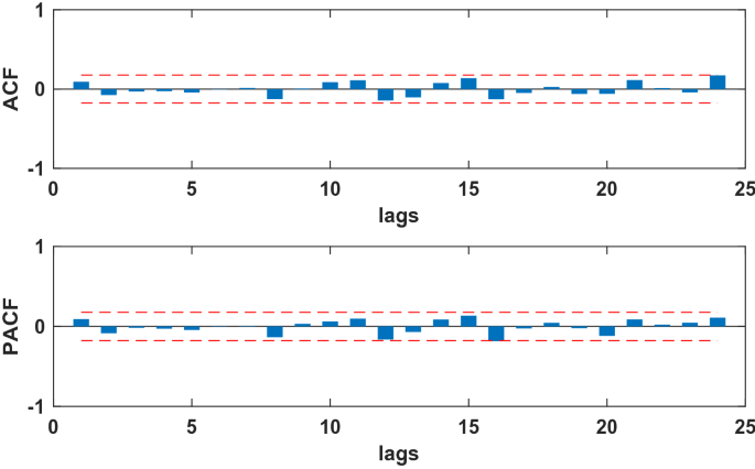
The ACF and PACF of residual sequence of the SARIMA((1,4,5,7),0,0)(0,1,2)₁₂ model.

The prediction analysis of NARNN model

We used the data of time series of human brucellosis cases from January 2008 to June 2020 in Xinjiang to train NARNN, 70% of the raw data was used as training data, 15% as validation data, and the remaining 15% as test data. By repeatedly adjusting the number of neurons in the hidden layer and the number of time lags, and finally, we found that the NARNN structure with 10 hidden layer neurons and 5 time lag was the best, and its error requirement was satisfied. The best validation performance was 13,464.0112 at epoch 6 (see Fig. 6). By using the established NARNN model to fit the original the number of monthly reported cases of human brucellosis, we got the graph of fitting and error results (see Fig. 7). The autocorrelation diagram of the errors was shown in Fig. 8. From Fig. 8, we could see that the error was only the largest correlation with itself, and the correlation coefficient at other lags was almost in the confidence interval, indicating that the established NARNN model had good fitting performance.

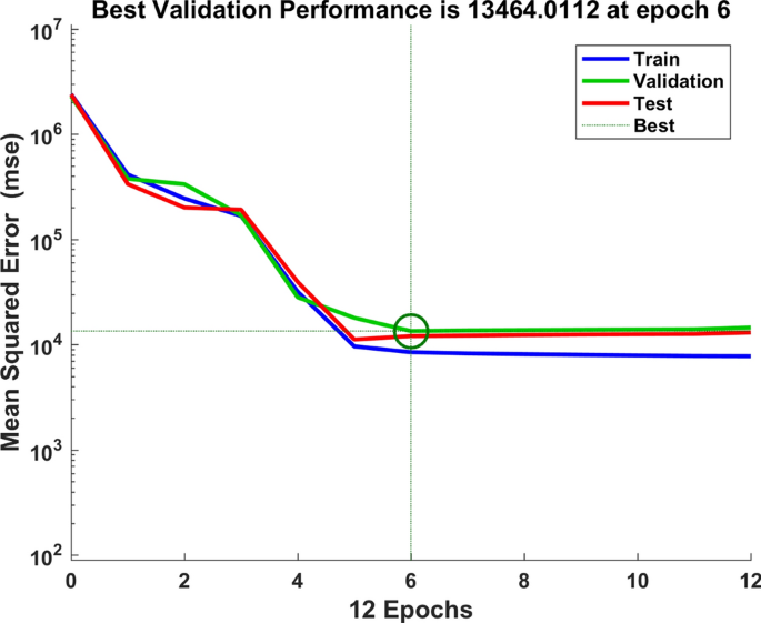
The graph of looking for the best validation performance.

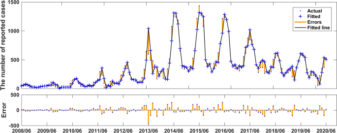
Actual series, fitted series, and residual series of the reported cases sequence of human brucellosis.

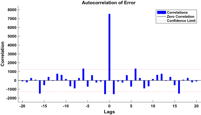
Autocorrelation graph of the residuals of the NARNN model.

Model comparison

Both the SARIMA((1,4,5,7),0,0)(0,1,2)₁₂ model and the established NARNN model in this study had good fitting performance and could be used to predict and analyze the number of reported cases of human brucellosis in the future. However, in order to obtain more accurate prediction values, we aimed to compare the two models and selected the better one to make prediction analysis. Therefore, we calculated the RMSE, MAE, and MAPE of the two models when they fitted the original human brucellosis sequence, respectively (see Table 3). From Table 3, we could see that the RMSE, MAE, and MAPE of the SARIMA((1,4,5,7),0,0)(0,1,2)₁₂ model were smaller than that of the NARNN model, indicating that the SARIMA((1,4,5,7),0,0)(0,1,2)₁₂ model was better than the established NARNN model. Therefore, the SARIMA((1,4,5,7),0,0)(0,1,2)₁₂ model was more suitable to predict the future number of human brucellosis cases in Xinjiang. We used the SARIMA((1,4,5,7),0,0)(0,1,2)₁₂ model to predict the number of reported cases of human brucellosis in Xinjiang from July 2020 to December 2021, as shown in Table 4. Furthermore, in order to see the performance of fitting and prediction more intuitively, we plotted the Fig. 9.

The SARIMA((1,4,5,7),0,0)(0,1,2)₁₂ model fitted and forecasted time series of reported cases of human brucellosis in Xinjiang.